Special Topics in GIS - M3.1 Scale Effect and Spatial Data Aggregation

 Scale determines the amount of data captured in spatial display, and as such it has direct effects on spatial properties of data. In both vector and raster data the smaller scale of measurement and the higher resolution, then the more data is available. 

On road polylines for example; roads and paths measured accurate to the nearest centimeter will contain much more data - more twists and odd jogs captured- than roads or walking paths measured to the nearest kilometer. In the kilometer scenario there may even be some paths excluded form the dataset altogether if they are under 0.5km in length. 

In a raster dataset this rule also holds true, but the effect of scale on spatial data is reflected more in the resolution -or cell size- of the raster. In rasters with large cell sizes less fine detail can be captured, so the data within each cell experiences an "averaging out" compared to rasters with smaller, finer resolution cells. This means that elevation properties like slope will decrease as the scale gets larger. This is not an inherently negative thing, as large scale and coarse resolution can be vital to displaying large areas in a short amount of time. It is important to keep in mind however how spatial properties can be manipulated by changing the scale and resolution of the data. 

Gerrymandering is one method used to manipulate data based on spatial properties. In this case the border of a voting district is drawn in such a way that the votes within it are more likely to be weighted in favor of certain demographics - even if those demographics don't make up the numerical majority of the area. By drawing the districts in these ways, representatives are effectively manipulating the scale of the votes in that area. Generally, districts that have been gerrymandered are not compact, and may divide communities or counties into different districts. By measuring compactness with a Polsby-Popper test (invented for paleontology and refined for politics by two lawyers in the 1990s) we can use area and perimeter to determine which districts are likely gerrymandered, and to what degree. 

During this analysis, I calculated the Polsby-Popper score for congressional districts in the continental Unites States, and highlighted those that were especially badly affected by a lack of compactness. 

This congressional district on the eastern seaboard is one of the worse "offenders" for not exhibiting compactness. The blue highlighted area outlines a district that wanders, doubles back on itself, and squeezes carefully in-between and around communities in order to manipulate scale of the votes in the district.  

Special Topics in GIS - M2.2 Interpolation

 For this assignment I used observed water quality points in Tampa Bay and a suite of interpolation techniques (Thiessen, IDW, and spline) to create a surface of water quality in Tampa Bay. 

Thiessen interpolation creates a series of polygons based on the spatial distribution of observed points, then fills each of those polygons with one value. Though this produces a very rough-scale result, it can be accomplished by hand if needed, and can be useful for quickly identifying entire regions at a time. For this analysis I used the Create Thiessen Polygons tool in conjunction with the Feature to Raster tool, which filled those polygons with values. 

Like Thiessen interpolation, Inverse Distance Weighted (IDW) interpolation is bound by the actual values entered, but uses the assumption that things close together must be more alike than things far away from eachother, and fills in the cells between values with estimates based on the nearby values. In IDW, values nearby are weighted higher for informing the estimated values. IDW creates a smooth raster that may contain hotspot-like nodes. The IDW analysis was easily completed by running the IDW tool on my existing datasets. 

Inverse distance weighted (IDW) interpolation of biological oxygen demand in Tamp Bay

Spline was the last technique examined, like IDW it takes existing values and creates estimates to fill the space between them, but where IDW uses a weight based on distance, Spline uses a constant weight from nearby points. The surface is "fitted" to the existing points as smoothly as possible, and the weight determines the allowable deviation. This means Spline may return values outside the range of the observed points, and will perform best with an evenly distributed sample set. 

Special Topics in GIS - M2.1 TIN and DEM

 In exploring and comparing the TIN and DEM data models, I -unsurprisingly perhaps- found DEM more familiar to work with. Based on previous experience in the UWF program and with displaying ecosystem data through my career, I felt like I had a better handle on how the DEM can be manipulated, which tools I had at my disposal, and consistent expectations for what the visual output would be from a given action. Though it is unfortunate that a DEM requires multiple calculations and tool runs to return values for aspect, slope, and elevation, I already had a solid foundation for this process. The neighbor-dependent nature of derived DEM values like this does produce a model that is easy to read, though less accurate than the TIN.

That being said, working with the TIN dataset for this project was extremely smooth, and as a researcher I think I prefer the higher accuracy available in the TIN, even if this somewhat sacrifices visual display for contour lines. The multiple faces of the triangle network in the TIN made it very clear when modeling difference values over a three dimensional structure, and I felt it was much quicker to get the necessary values in the TIN for aspect, slope, and elevation than the successive familiar tool running with the DEM. 

Overall, while I would be more likely to use a DEM for a public-facing map or display, I appreciate the data quality advantages of the TIN model. When working with three dimensional elevation data especially, I think it will be my first choice whenever one is available. 

A screenshot of the DEM model, with layers of calculated DEMs visible in the contents pane. TINs do not require these additional calculations to display the same information. 

Special Topics in GIS - M1.3 Assessment

The goal of an accuracy assessment is to help determine how reliable data is compared to the "actual" - or as close as can be reasonably determined as the actual. With the standardized techniques in the National Standard for Spatial Data Accuracy (NSSDA), we get a determination of positional accuracy that can be used to quantify how "off" a geospatial dataset is from the actual. With standardized protocols like this the accuracy statements become comparable to one another between datasets, allowing a user to select data that meets their needs for this aspect of data quality.

In the NSSDA protocol, the horizontal or vertical distance between a subset (>=20) of dataset features and the "actual" location of the feature is compared, and the difference between the actual and the dataset coordinates are then squared, summed, averaged with mean, and square-rooted to return the Root Mean Square Error. This error is then multiplied by a standard value that represents the average amount of error in the 95th percentile for horizontal or vertical data. The result is the shortest distance in the dataset that can be "trusted", expressed as an accuracy statement to the 95th percentile. 

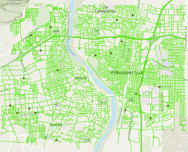
For this lab a different aspect of data quality was examined; completeness. If accuracy helps determine if a dataset can be used based on how "trustworthy" it is, then completeness determines if a dataset can be used based on the amount of information it contains. In this lab, the completeness of two street datasets was assessed based on amount of data. The street polylines were overlaid and assessed with a grid. This method highlighted areas where the county-provided shapefile contained more lines (reds) and areas where the US Census' Topologically Integrated Geographic Encoding and Referencing (TIGER) dataset contained more lines (blues).

Red areas where the Jackson County file contained more road and blue areas where the TIGER dataset contained more road.

Special Topics in GIS - M1.2 Standards

Reference points representing the "true" location of intersections.

As previously discussed, to determine accuracy a datapoint must be compared to a known reference point for what the "true" value is. In this project the goal was to compare the accuracy of two polyline street datasets; one from the City of Albuquerque, and one from the company StreetMap USA. The reference points were determined by using raster satellite images of the roads and neighborhoods contained in both polyline datasets. I selected 20 reference points at intersections throughout the sample area based on guidelines in the Positional Accuracy Handbook. After that I created point datasets that corresponded with the location of those same intersections in each of the street polyline sets. From here, each of the street datasets could be compared with the "true" location of the intersection. I imported the coordinate values into Excel to run the RMSE, and determine the NSSDA for horizontal accuracy of each street dataset. 

Horizontal positional accuracy: 

Using the National Standard for Spatial Data Accuracy, the City data set tested 24.8 feet horizontal accuracy at 95% confidence level.

Using the same National Standard for Spatial Data Accuracy, the StreetMap USA data set tested 278.1 feet horizontal accuracy at 95% confidence level.

Special Topics in GIS - M1.1 Fundementals

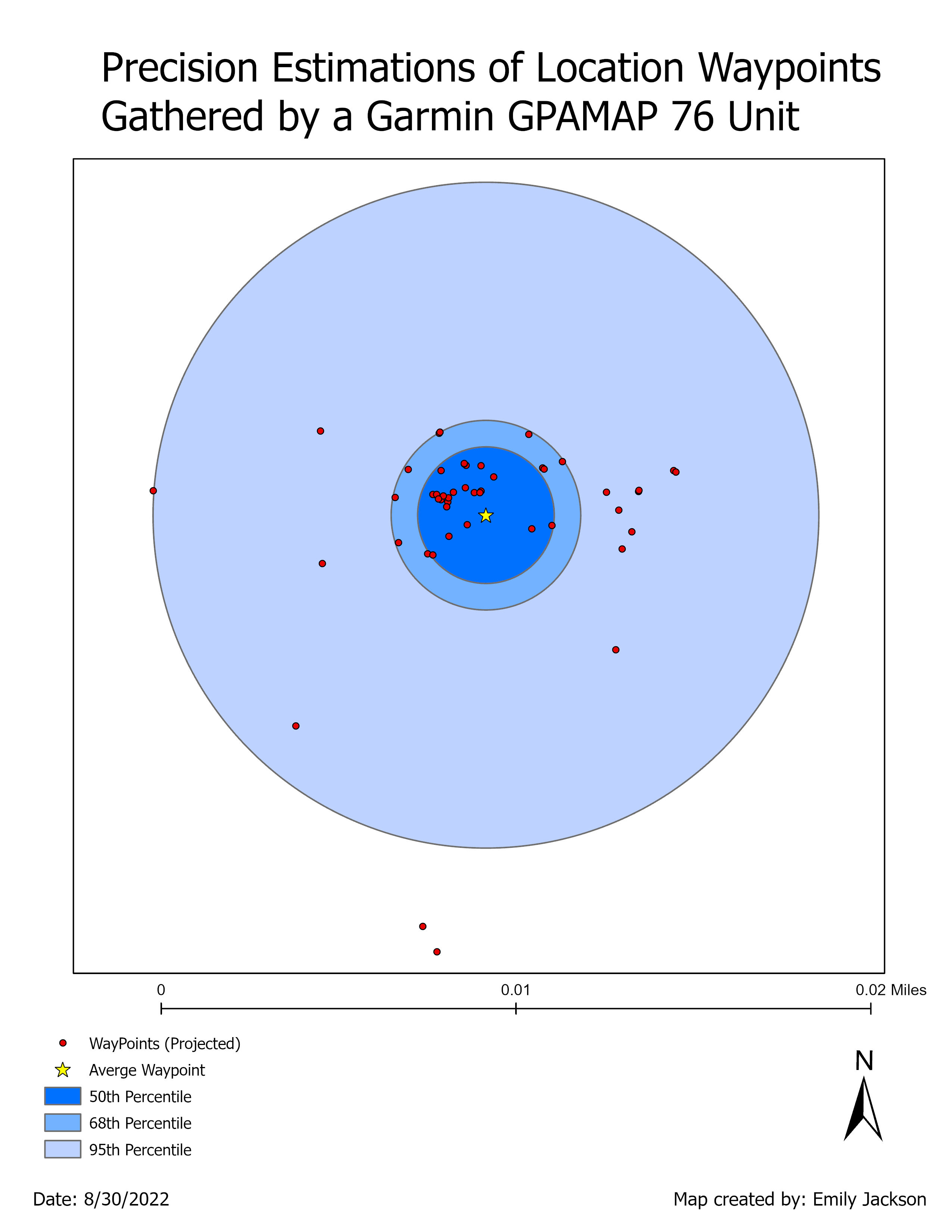
The precision of waypoints mapped by the Garmin GPSMap 76. Blue buffers denote 50th, 68th, and 95th percentiles, the star is the calculated mean waypoint location. 

A primary tenant of mapping and analyzing data well is the ability to assess whether you are working with good data in the first place. For the first lab in Special Topics, we reviewed the fundamentals of data accuracy and precision, particularly in regard to the horizontal and vertical attributes often associated with GIS location data.

The dataset we worked with was 50 points taken several years ago around a single location by a Garmin GPSMap 76. Through basic geospatial and statistical analysis I determined the horizontal and vertical accuracy and precision for the dataset. A subset of those determinations are below:

Horizontal accuracy: 3.49 meters                        Horizontal precision: 4.3 meters

Horizontal accuracy is determined by comparing the waypoints to a known reference point. This is effectively a measurement of how far "off" from the actual xy point the mapping unit was recording locations. Horizontal precision however is a measurement of the range of values returned by the unit, and does not require the "actual" xy point because it is a comparison of waypoints to one another. To determine precision in this case I calculated an average xy coordinate from the waypoint data, then compared how far away from that mean each of the other waypoints were.